Change Coordinates!
Introduction
Hello, I am Greg Graviton, this is our new blog, and this is my first post which is going to be about the usefulness of changes of coordinates.
My goal is to write about Hamiltonian Mechanics and symplectic geometry, but we need some prerequisites in differential geometry for that. Hence, I’m planning a series of introductory posts, beginning with this one which tackles the key idea of change of coordinates and coordinate independence.
This is a very general and useful concept to have in your toolbox; for instance, it subsumes eigenvalues and it’s the very foundation of differential geometry.
Now, I’m not going to write a standard textbook introduction to differential geometry here. Rather, I would like to present it as a small mathematical gem: lightweight and delightful, with a focus on examples and key ideas instead of systematic textbook development, for the latter all too often obscures the former.
Solving ordinary differential equations (ODEs)
Two masses connected by a spring
As a first example, consider two masses connected by a spring. For simplicity, we assume that the masses are equal 


By Newton’s laws, the equations of motion are

where 


So, now, uh, how do we solve this? I mean, single equations like 

The key idea is that

Clearly, the coordinates 


But more importantly, these new quantities now fulfill the differential equations

which are no longer coupled and can be solved independently! For instance, the solution to the first is clearly 
Eigenvalues
Let’s ramp difficulty up a bit and consider a general linear system of differential equations

essentially given by a matrix 

How to solve that? Previously, the center of mass was a very useful coordinate, but since
The idea here is to simply consider all possible changes of coordinates at once and pick the one that works best. More precisely, we make the ansatz of a linear change of coordinates given by a matrix 

and hope that we can find a good 
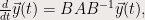
so we want 
Hence, if you know how to calculate eigenvalues, you can solve differential equations.
Variation of constants
Let’s be even more general and consider an inhomogenous linear system of differential equations where the coefficients may now depend on

How to solve that? Well, in general, it won’t be possible to calculate an analytic solution. But suppose that we can somehow solve the corresponding homogenous problem
(Homogenous
means that the sum of two solutions is again a solution, and that we can multiply a solution with a constant 

of a set of 


that replaces the constants 

I never understood how this mysterious procedure of varying things that are supposed to be constant works, until I realized that it’s actually a change of coordinates! I mean, we want to calculate 

But why should there be anything special about the standard basis vectors 

In contrast, the 
Integration
Calculating integrals is another prime example for the power of coordinate changes. If you have ever calculated a multi-dimensional integral, you probably know about coordinate systems different from the usual cartesian one, like polar or spherical coordinates.
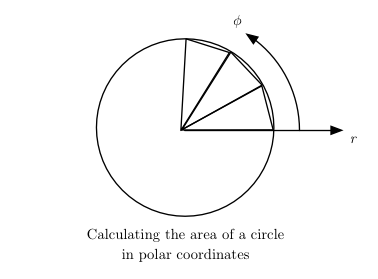
For instance, consider the area of the unit circle. In cartesian coordinates 

But that’s the fault of the cartesian coordinates, they simply don’t reflect the symmetries of a circle as you can see from the picture.

In contrast, polar coordinates are much more suitable and give

immediately, with the caveat that the volume element is now 

Conclusion
I hope that these examples have demonstrated the usefulness of changes of coordinates; a technique which is, in a sense, pervasive to mathematics and physics.
Now, to foreshadow future blog posts, if differential equations and integration are best solved by changing coordinates, how about describing these problems in a coordinate independent fashion, i.e. without mentioning coordinates in the first place, so that we are free to pick a good set of coordinates later on?
This question is one of the starting point for differential geometry and the mathematics of manifolds. For instance, the coordinate independent formulation of ordinary differential equations is given by vector fields, and the so-called differential forms are the key ingredient to coordinate-free integrals.
This geometric approach is also taken by V.I. Arnold’s marvelous book “Ordinary differential equations”, which for example also mentions the interpretation of the variation of constants as a coordinate change. Highly recommended!
Next time, I intend to write about vector fields and their coordinate-free description.
